


Practical Machine Learning with Python and Keras
Table of Contents
- What is machine learning, and why do we care?
- Supervised machine learning
- Understanding Artificial Neural Networks
- Using the Keras library to train a simple Neural Network that recognizes handwritten digits
- Running the iPython Notebook Locally
- Running from a Minimal Python Distribution
- The MNIST Dataset
- The objective
- The dataset
- Reading the labels
- Reading the images
- Encoding image labels using one-hot encoding
- Training a Neural Network using Keras
- Inspecting the results
- Understanding the output of a softmax activation layer
- Reading the output of a softmax activation layer for our digit
- Viewing the confusion matrix
- Conclusion
- Take home exercise
What is machine learning, and why do we care?
Machine learning is a field of artificial intelligence that uses statistical techniques to give computer systems the ability to “learn” (e.g., progressively improve performance on a specific task) from data, without being explicitly programmed. Think of how efficiently (or not) Gmail detects spam emails, or how good text-to-speech has become with the rise of Siri, Alexa, and Google Home.
Some of the tasks that can be solved by implementing Machine Learning include:
- Anomaly and fraud detection: Detect unusual patterns in credit card and bank transactions.
- Prediction: Predict future prices of stocks, exchange rates, and now cryptocurrencies.
- Image recognition: Identify objects and faces in images.
Machine Learning is an enormous field, and today we’ll be working to analyze just a small subset of it.
Supervised Machine Learning
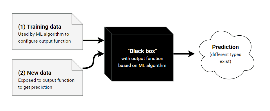
Supervised learning is one of Machine Learning’s subfields. The idea behind Supervised Learning is that you first teach a system to understand your past data by providing many examples to a specific problem and desired output. Then, once the system is “trained”, you can show it new inputs in order to predict the outputs.
How would you build an email spam detector? One way to do it is through intuition – manually defining rules that make sense: such as “contains the word money”, or “contains the word ‘Western Union’”. While manually built rule-based systems can work sometimes, others it becomes hard to create or identify patterns and rules based only on human intuition. By using Supervised Learning, we can train systems to learn the underlying rules and patterns automatically with a lot of past spam data. Once our spam detector is trained, we can feed it new a new email so that it can predict how likely an email is a spam.
Earlier I mentioned that you can use Supervised Learning to predict an output. There are two primary kinds of supervised learning problems: regression and classification.
- In regression problems, we try to predict a continuous output. For example, predicting the price (real value) of a house when given its size.
- In classification problems, we try to predict a discrete number of categorical labels. For example, predicting if an email is spam or not given the number of words within it.
You can’t talk about Supervised Machine Learning without talking about supervised learning models – it’s like talking about programming without mentioning programming languages or data structures. In fact, the learning models are the structures that are “trained,” and their weights or structure change internally as they mold and understand what we are trying to predict. There are plenty of supervised learning models, some of the ones I have personally used are:
- Random Forest
- Naive Bayes
- Logistic Regression
- K Nearest Neighbors
Today we’ll be using Artificial Neural Networks (ANNs) as our model of choice.
Understanding Artificial Neural Networks
ANNs are named this way because their internal structure is meant to mimic the human brain. A human brain consists of neurons and synapses that connect these neurons with each other, and when these neurons are stimulated, they “activate” other neurons in our brain through electricity.
In the world of ANNs, each neuron is “activated” by first computing the weighted sum of its incoming inputs (other neurons from the previous layer), and then running the result through activation function. When a neuron is activated, it will, in turn, activate other neurons that will perform similar computations, causing a chain reaction between all the neurons of all the layers.
It’s worth mentioning that, while ANNs are inspired by biological neurons, they are in no way comparable.

- What the diagram above is describing here is the entire activation process that every neuron goes through. Let’s look at it together from left to right.
- All the inputs (numerical values) from the incoming neurons are read. The incoming inputs are identified as x1..xn
- Each input is multiplied by the weight associated with that connection. The weights associated with the connections here are denoted as W1j..Wnj.
- All the weighted inputs are summed together and passed into the activation function. The activation function reads the single summed weighted input and transforms it into a new numerical value.K Nearest Neighbors
- Finally, the numerical value that was returned by the activation function will then be the input of another neuron in another layer.
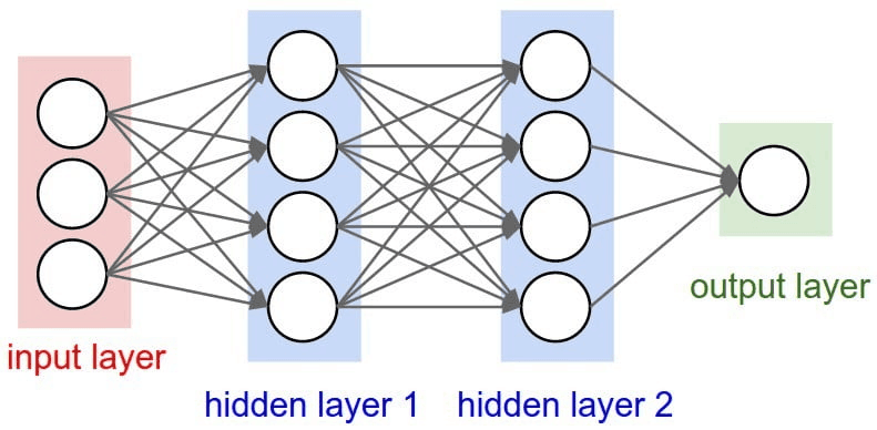
Neural Network layers
Neurons inside the ANN are arranged into layers. Layers are a way to give structure to the Neural Network, each layer will contain 1 or more neurons. A Neural Network will usually have 3 or more layers. There are 2 special layers that are always defined, which are the input and the output layer.
- The input layer is used as an entry point to our Neural Network. In programming, think of this as the arguments we define to a function.
- The output layer is used as the result to our Neural Network. In programming, think of this as the return value of a function.
The layers in between are described as “hidden layers”, and they are where most of the computation happens. All layers in an ANN are encoded as feature vectors.
Choosing how many hidden layers and neurons
There isn’t necessarily a golden rule on choosing how many layers and their size (or the number of neurons they have). Generally, you want to try and at least have 1 hidden layer and tweak around the size to see what works best.
Using the Keras library to train a simple Neural Network that recognizes handwritten digits
For us Python Software Engineers, there’s no need to reinvent the wheel. Libraries like Tensorflow, Torch, Theano, and Keras already define the main data structures of a Neural Network, leaving us with the responsibility of describing the structure of the Neural Network in a declarative way.
Keras gives us a few degrees of freedom here: the number of layers, the number of neurons in each layer, the type of layer, and the activation function. In practice, there are many more of these, but let’s keep it simple. As mentioned above, there are two special layers that need to be defined based on your problematic domain: the size of the input layer and the size of the output layer. All the remaining “hidden layers” can be used to learn the complex non-linear abstractions to the problem.
Today we’ll be using Python and the Keras library to predict handwritten digits from the MNIST dataset. There are three options to follow along: use the rendered Jupyter Notebook hosted on Kite’s github repository, running the notebook locally, or running the code from a minimal python installation on your machine.
Running the iPython Notebook Locally
If you wish to load this Jupyter Notebook locally instead of following the linked rendered notebook, here is how you can set it up:
Requirements:
- A Linux or Mac operating system
- Conda 4.3.27 or later
- Git 2.13.0 or later
- wget 1.16.3 or later
In a terminal, navigate to a directory of your choice and run:
# Clone the repository

git clone https://github.com/kiteco/kite-python-blog-post-code.git

cd kite-python-blog-post-code/Practical\ Machine\ Learning\ with\ Python\ and\ Keras/


# Use Conda to setup and activate the Python environment with the correct  dependencies

conda env create -f environment.yml

source activate kite-blog-post
Running from a Minimal Python Distribution
To run from a pure Python installation (anything after 3.5 should work), install the required modules with pip, then run the code as typed, excluding lines marked with a % which are used for the iPython environment.
It is strongly recommended, but not necessary, to run example code in a virtual environment. For extra help, see https://packaging.python.org/guides/installing-using-pip-and-virtualenv/
# Set up and Activate a Virtual Environment under Python3


$ pip3 install virtualenv

$ python3 -m virtualenv venv

$ source venv/bin/activate


# Install Modules with pip (not pip3)


(venv) $ pip install matplotlib

(venv) $ pip install sklearn

(venv) $ pip install tensorflow
Okay! If these modules installed successfully, you can now run all the code in this project.
In [1]:
import numpy as np

import matplotlib.pyplot as plt

import gzip

from typing import List

from sklearn.preprocessing import OneHotEncoder

import tensorflow.keras as keras

from sklearn.model_selection import train_test_split

from sklearn.metrics import confusion_matrix

import itertools

%matplotlib inline
The MNIST Dataset
The MNIST dataset is a large database of handwritten digits that is used as a benchmark and an introduction to machine learning and image processing systems. We like MNIST because the dataset is very clean and this allows us to focus on the actual network training and evaluation. Remember: a clean dataset is a luxury in the ML world! So let’s enjoy and celebrate MNIST’s cleanliness while we can 🙂
The objective
Given a dataset of 60,000 handwritten digit images (represented by 28×28 pixels, each containing a value 0 – 255 with its grayscale value), train a system to classify each image with it’s respective label (the digit that is displayed).
The dataset
The dataset is composed of a training and testing dataset, but for simplicity we are only going to be using the training set. Below we can download the train dataset
In [2]:
%%bash

rm -Rf train-images-idx3-ubyte.gz

rm -Rf train-labels-idx1-ubyte.gz

wget -q http://yann.lecun.com/exdb/mnist/train-images-idx3-ubyte.gz

wget -q http://yann.lecun.com/exdb/mnist/train-labels-idx1-ubyte.gz
Reading the labels
There are 10 possible handwritten digits: (0-9), therefore every label must be a number from 0 to 9. The file that we downloaded, train-labels-idx1-ubyte.gz, encodes labels as following:
TRAINING SET LABEL FILE (train-labels-idx1-ubyte):
| [offset] | [type] | [value] | [description] |
| 0000 | 32 bit integer | 0x00000801(2049) | magic number (MSB first) |
| 0004 | 32 bit integer | 60000 | number of items |
| 0008 | unsigned byte | ?? | label |
| 0009 | unsigned byte | ?? | label |
| ….. | ….. | ….. | ….. |
| xxxx | unsigned byte | ?? | label |
The labels values are 0 to 9.
It looks like the first 8 bytes (or the first 2 32-bit integers) can be skipped because they contain metadata of the file that is usually useful to lower-level programming languages. To parse the file, we can perform the following operations:
- Open the file using the gzip library, so that we can decompress the file
- Read the entire byte array into memory
- Skip the first 8 bytes
- Iterate over every byte, and cast that byte to integer
NOTE: If this file was not from a trusted source, a lot more checking would need to be done. For the purpose of this blog post, I’m going to assume the file is valid in it’s integrity.
In [3]:
with gzip.open('train-labels-idx1-ubyte.gz') as train_labels:

    data_from_train_file = train_labels.read()


# Skip the first 8 bytes, we know exactly how many labels there are

label_data = data_from_train_file[8:]

assert len(label_data) == 60000


# Convert every byte to an integer. This will be a number between 0 and 9

labels = [int(label_byte) for label_byte in label_data]

assert min(labels) == 0 and max(labels) == 9

assert len(labels) == 60000
Reading the images
| [offset] | [type] | [value] | [description] |
| 0000 | 32 bit integer | 0x00000803(2051) | magic number |
| 0004 | 32 bit integer | 60000 | number of images |
| 0008 | 32 bit integer | 28 | number of rows |
| 0012 | 32 bit integer | 28 | number of columns |
| 0016 | unsigned byte | ?? | pixel |
| 0017 | unsigned byte | ?? | pixel |
| ….. | ….. | ….. | ….. |
| xxxx | unsigned byte | ?? | pixel |
Reading images is slightly different than reading labels. The first 16 bytes contain metadata that we already know. We can skip those bytes and directly proceed to reading the images. Every image is represented as a 28*28 unsigned byte array. All we have to do is read one image at a time and save it into an array.
In [4]:
SIZE_OF_ONE_IMAGE = 28 ** 2

images = []


# Iterate over the train file, and read one image at a time

with gzip.open('train-images-idx3-ubyte.gz') as train_images:

    train_images.read(4 * 4)

    ctr = 0

    for _ in range(60000):

        image = train_images.read(size=SIZE_OF_ONE_IMAGE)

        assert len(image) == SIZE_OF_ONE_IMAGE


        # Convert to numpy

        image_np = np.frombuffer(image, dtype='uint8') / 255

        images.append(image_np)


images = np.array(images)

images.shape
Out [4]: (60000, 784)
Our images list now contains 60,000 images. Each image is represented as a byte vector of SIZE_OF_ONE_IMAGE Let’s try to plot an image using the matplotlib library:
In [5]:
def plot_image(pixels: np.array):

    plt.imshow(pixels.reshape((28, 28)), cmap='gray')

    plt.show()

plot_image(images[25])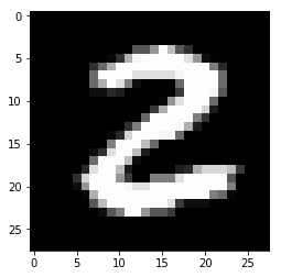
Encoding image labels using one-hot encoding
We are going to use One-hot encoding to transform our target labels into a vector.
In [6]:
labels_np = np.array(labels).reshape((-1, 1))


encoder = OneHotEncoder(categories='auto')

labels_np_onehot = encoder.fit_transform(labels_np).toarray()


labels_np_onehot
Out [6]:
array([[0., 0., 0., ..., 0., 0., 0.],

       [1., 0., 0., ..., 0., 0., 0.],

       [0., 0., 0., ..., 0., 0., 0.],

       ...,

       [0., 0., 0., ..., 0., 0., 0.],

       [0., 0., 0., ..., 0., 0., 0.],

       [0., 0., 0., ..., 0., 1., 0.]])
We have successfully created input and output vectors that will be fed into the input and output layers of our neural network. The input vector at index i will correspond to the output vector at index i
In [7]:
labels_np_onehot[999]
Out [7]:
array([0., 0., 0., 0., 0., 0., 1., 0., 0., 0.])
In [8]:
plot_image(images[999])

In the example above, we can see that the image at index 999 clearly represents a 6. It’s associated output vector contains 10 digits (since there are 10 available labels) and the digit at index 6 is set to 1, indicating that it’s the correct label.
Building train and test split
In order to check that our ANN has correctly been trained, we take a percentage of the train dataset (our 60,000 images) and set it aside for testing purposes.
In [9]:
X_train, X_test, y_train, y_test = train_test_split(images, labels_np_onehot)
In [10]:
y_train.shape
Out [10]:
(45000, 10)
In [11]:
y_test.shape
Out [11]:
(15000, 10)
As you can see, our dataset of 60,000 images was split into one dataset of 45,000 images, and the other of 15,000 images.
Training a Neural Network using Keras
In [12]:
model = keras.Sequential()

model.add(keras.layers.Dense(input_shape=(SIZE_OF_ONE_IMAGE,), units=128, activation='relu'))

model.add(keras.layers.Dense(10, activation='softmax'))


model.summary()


model.compile(optimizer='sgd',

              loss='categorical_crossentropy',

metrics=['accuracy'])| Layer (type) | Output Shape | Param # |
| dense (Dense) | (None, 128) | 100480 |
| dense_1 (Dense) | (None, 10) | 1290 |
Total params: 101,770
Trainable params: 101,770
Non-trainable params: 0
In [13]:
X_train.shape
Out [13]:
(45000, 784)
In [14]:
model.fit(X_train, y_train, epochs=20, batch_size=128)
Epoch 1/20

45000/45000 [==============================] - 8s 169us/step - loss: 1.3758 - acc: 0.6651

Epoch 2/20

45000/45000 [==============================] - 7s 165us/step - loss: 0.6496 - acc: 0.8504

Epoch 3/20

45000/45000 [==============================] - 8s 180us/step - loss: 0.4972 - acc: 0.8735

Epoch 4/20

45000/45000 [==============================] - 9s 191us/step - loss: 0.4330 - acc: 0.8858

Epoch 5/20

45000/45000 [==============================] - 8s 186us/step - loss: 0.3963 - acc: 0.8931

Epoch 6/20

45000/45000 [==============================] - 8s 183us/step - loss: 0.3714 - acc: 0.8986

Epoch 7/20

45000/45000 [==============================] - 8s 182us/step - loss: 0.3530 - acc: 0.9028

Epoch 8/20

45000/45000 [==============================] - 9s 191us/step - loss: 0.3387 - acc: 0.9055

Epoch 9/20

45000/45000 [==============================] - 8s 175us/step - loss: 0.3266 - acc: 0.9091

Epoch 10/20

45000/45000 [==============================] - 9s 199us/step - loss: 0.3163 - acc: 0.9117

Epoch 11/20

45000/45000 [==============================] - 8s 185us/step - loss: 0.3074 - acc: 0.9140

Epoch 12/20

45000/45000 [==============================] - 10s 214us/step - loss: 0.2991 - acc: 0.9162

Epoch 13/20

45000/45000 [==============================] - 8s 187us/step - loss: 0.2919 - acc: 0.9185

Epoch 14/20

45000/45000 [==============================] - 9s 202us/step - loss: 0.2851 - acc: 0.9203

Epoch 15/20

45000/45000 [==============================] - 9s 201us/step - loss: 0.2788 - acc: 0.9222

Epoch 16/20

45000/45000 [==============================] - 9s 206us/step - loss: 0.2730 - acc: 0.9241

Epoch 17/20

45000/45000 [==============================] - 7s 164us/step - loss: 0.2674 - acc: 0.9254

Epoch 18/20

45000/45000 [==============================] - 9s 189us/step - loss: 0.2622 - acc: 0.9271

Epoch 19/20

45000/45000 [==============================] - 10s 219us/step - loss: 0.2573 - acc: 0.9286

Epoch 20/20

45000/45000 [==============================] - 9s 197us/step - loss: 0.2526 - acc: 0.9302
Out [14]:
<tensorflow.python.keras.callbacks.History at 0x1129f1f28>>
In [15]:
model.evaluate(X_test, y_test)
15000/15000 [==============================] – 2s 158us/step
Out [15]:
[0.2567395991722743, 0.9264]
Inspecting the results
Congratulations! you just trained a neural network to predict handwritten digits with more than 90% accuracy! Let’s test out the network with one of the pictures we have in our testset
Let’s take a random image, in this case the image at index 1010. We take the predicted label (in this case, the value is a 4 because the 5th index is set to 1)
In [16]:
y_test[1010]
Out [16]:
array([0., 0., 0., 0., 1., 0., 0., 0., 0., 0.])
Let’s plot the image of the corresponding image
In [17]:
plot_image(X_test[1010])

Understanding the output of a softmax activation layer
Now, let’s run this number through the neural network and we can see what our predicted output looks like!
In [18]:
predicted_results = model.predict(X_test[1010].reshape((1, -1)))
The output of a softmax layer is a probability distribution for every output. In our case, there are 10 possible outputs (digits 0-9). Of course, every one of our images is expected to only match one specific output (in other words, all of our images only contain one distinct digit).
Because this is a probability distribution, the sum of the predicted results is ~1.0
In [19]:
predicted_results.sum()
Out [19]:
1.0000001
Reading the output of a softmax activation layer for our digit
As you can see below, the 7th index is really close to 1 (0.9) which means that there is a 90% probability that this digit is a 6… which it is! congrats!
In [20]:
predicted_results
Out [20]:
array([[1.2202066e-06, 3.4432333e-08, 3.5151488e-06, 1.2011528e-06,

        9.9889344e-01, 3.5855610e-05, 1.6140550e-05, 7.6822333e-05,

        1.0446112e-04, 8.6736667e-04]], dtype=float32)
Viewing the confusion matrix
In [21]:
predicted_outputs = np.argmax(model.predict(X_test), axis=1)

expected_outputs = np.argmax(y_test, axis=1)


predicted_confusion_matrix = confusion_matrix(expected_outputs, predicted_outputs)
In [22]:
predicted_confusion_matrix
Out [22]:
array([[1413,    0,   10,    3,    2,   12,   12,    2,   10,    1],

       [   0, 1646,   12,    6,    3,    8,    0,    5,    9,    3],

       [  16,    9, 1353,   16,   22,    1,   18,   28,   44,    3],

       [   1,    6,   27, 1420,    0,   48,   11,   16,   25,   17],

       [   3,    7,    5,    1, 1403,    1,   12,    3,    7,   40],

       [  15,   13,    7,   36,    5, 1194,   24,    6,   18,   15],

       [  10,    8,    9,    1,   21,   16, 1363,    0,    9,    0],

       [   2,   14,   18,    4,   16,    4,    2, 1491,    1,   27],

       [   4,   28,   19,   31,   10,   28,   13,    2, 1280,   25],

       [   5,   13,    1,   21,   58,   10,    1,   36,   13, 1333]])
In [23]:
# Source code: https://scikit-learn.org/stable/auto_examples/model_selection/plot_confusion_matrix.html

def plot_confusion_matrix(cm, classes,

                          title='Confusion matrix',

                          cmap=plt.cm.Blues):

    """

    This function prints and plots the confusion matrix.

    Normalization can be applied by setting `normalize=True`.

    """


    plt.imshow(cm, interpolation='nearest', cmap=cmap)

    plt.title(title)

    plt.colorbar()

    tick_marks = np.arange(len(classes))

    plt.xticks(tick_marks, classes, rotation=45)

    plt.yticks(tick_marks, classes)


    fmt = 'd'

    thresh = cm.max() / 2.

    for i, j in itertools.product(range(cm.shape[0]), range(cm.shape[1])):

        plt.text(j, i, format(cm[i, j], fmt),

                 horizontalalignment="center",

                 color="white" if cm[i, j] > thresh else "black")


    plt.ylabel('True label')

    plt.xlabel('Predicted label')

    plt.tight_layout()


# Compute confusion matrix

class_names = [str(idx) for idx in range(10)]

cnf_matrix = confusion_matrix(expected_outputs, predicted_outputs)

np.set_printoptions(precision=2)


# Plot non-normalized confusion matrix

plt.figure()

plot_confusion_matrix(cnf_matrix, classes=class_names,

                      title='Confusion matrix, without normalization')


plt.show()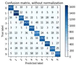
Conclusion
During this tutorial, you’ve gotten a taste of a couple important concepts that are a fundamental part of one’s job in Machine Learning. We learned how to:
- Encode and decode images in the MNIST dataset
- Encode categorical features using one-hot encoding
- Define our Neural Network with 2 hidden layers, and an output layer that uses the softmax activation function
- Inspect the results of a softmax activation function output
- Plot the confusion matrix of our classifier
Libraries like Sci-Kit Learn and Keras have substantially lowered the entry barrier to Machine Learning – just as Python has lowered the bar of entry to programming in general. Of course, it still takes years (or decades) of work to master!
Engineers who understand Machine Learning are in strong demand. With the help of the libraries I mentioned above, and introductory blog posts focused on Practical machine learning (like this one), all engineers should be able to get their hands on Machine Learning even if they don’t understand the full theoretical reasoning behind a particular model, library, or framework. And, hopefully, they’ll use this skill to improve whatever they’re building every day.
If we start making our components a little bit smarter and a little more personalized every day, we can make customers more engaged and at the center of whatever we are building.
Take home exercise
In my next article, I’ll be showing you how to deploy a learning model using gRPC and Docker. But in the meantime, here are a few challenges you can do at home to dig deeper into the world of machine learning using Python:
- Tweak around with the number of neurons in the hidden layer. Can you increase the accuracy?
- Try to add more layers. Does the neural network train slower? Can you think of why?
- Try to train a Random Forest classifier (requires scikit-learn library) instead of a Neural Network. Is the accuracy better?
This post is a part of Kite’s new series on Python. You can check out the code from this and other posts on our GitHub repository.
Resources
 in San Francisco